Classify Iris Flowers using R and R Shiny

This tutorial is designed to show you how to get started using R in cnvrg. Following this tutorial will also give you insights into some of the advanced features of cnvrg.

We will be specifically covering the following features of cnvrg:

• Launching R Studio
• Running an experiment
• Running a grid search
• Comparing experiments

About Iris

This project is based around analyzing a famous dataset of 150 images or iris flowers. The goal is to use the labelled attributes accompanying the images to learn to distinguish between different types of iris flowers.

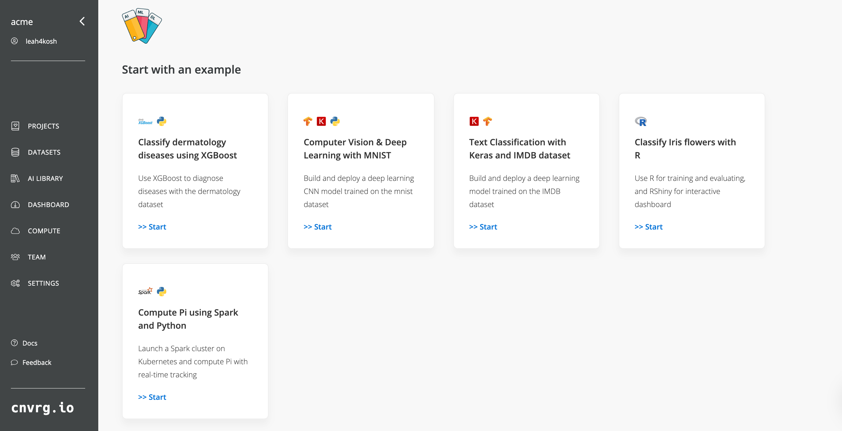
Getting the project started

On the website, navigate to the Projects tab.

Welcome to the home of your code, experiments, flows and deployments. Here everything lives and works together.

For this example, we’ll use the prebuilt example project. On the top right, click Example Projects.

Select Classify Iris flowers with R.

Now you’ve created a cnvrg project titled iris. The iris project dashboard is displayed. Let’s have a closer look at what’s inside the project and files.

Launching an R Studio workspace

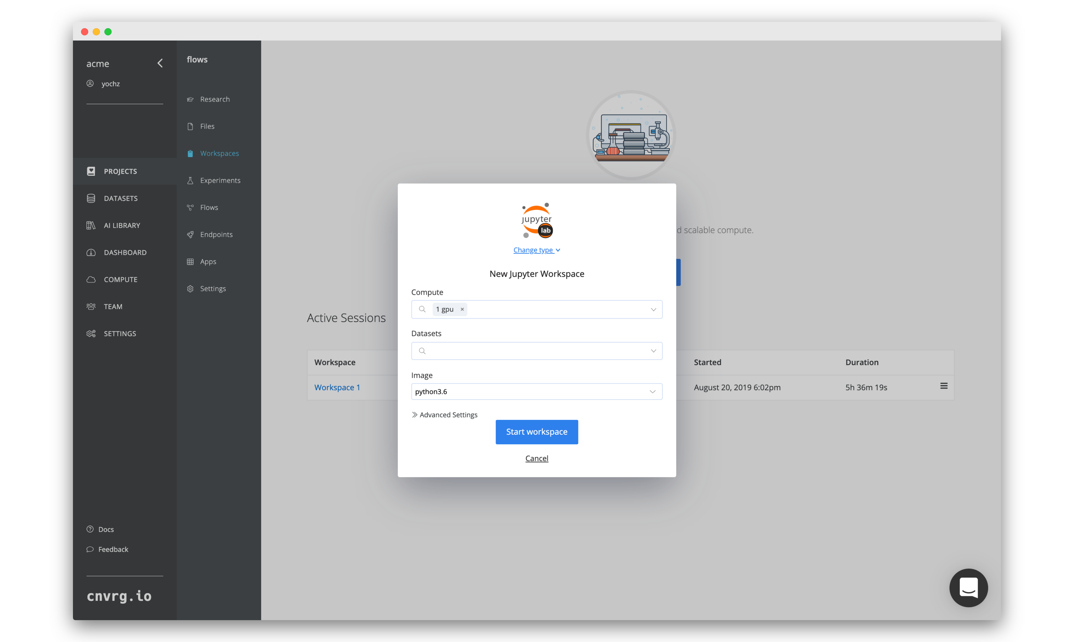
On the current page, click the Start New Workspace.

TIP

You can always make new workspaces through the Workspaces tab on the sidebar.

Now let’s fill in this form to get our R Studio notebook up and running. By default, the workspace type is Jupyter lab, so we will need to select R Studio.

1. Click Change Tyoe and then click R Studio.
2. For Compute, select medium (running on Kubernetes).
3. Leave Datasets empty.
4. For Image, click cnvrg_r and choose the latest cnrvg R image.
5. Click Start workspace.

cnvrg will now put everything into motion and get a R Studio workspace up and running for us to use. It may take a few moments but soon enough, everything will be ready to go.

This is how it looks:

With the notebook, you can run code and play around with your data to better design your models. You can also open and edit your code. For example, we can open train.R and have a look at the code that our example project has provided. Any changes you make will be committed using cnvrg’s built-in version management.

Model Tracking and Visualization

---

One of cnvrg’s great features is Research Assistant. Using a simple print to stdout, Research Assistant lets cnvrg automatically track any metrics you want. You can then easily compare experiments and models later on.

The format is as follows:

(‘<cnrvg_tag_NAME>’, keyvalue)

Research Assistant will automatically keep track of these and present them to you for easy comprehension. The train.R file already has these added. Take a look at lines 26-31:

# Print cnvrg Research tags for the Parameters
cat(sprintf("cnvrg_tag_partition_size: %f\n", opt$partition_size));
cat(sprintf("cnvrg_tag_folds: %d\n", opt$folds));

# Use folds to set experiment title
cat(sprintf("cnvrg_experiment_title: Experiment using %d folds\n", opt$folds));

These line will track the partition_size and folds as tags for the experiment.

Great! Let’s train our new model in an experiment.

WARNING

Make sure you click Sync to keep the changes up to date!

Experiments

Experiments are the core of every machine learning project. When building a model, it’s all about trying new ideas, testing new hypotheses, testing hyperparameters, and exploring different neural-network architecture.

At cnvrg, we help you to experiment 10x faster and get everything 100% reproducible and trackable, so you can focus on the important stuff.

An experiment is basically a “run” of a script, locally or remotely. Usually, to run an experiment on a remote GPU, you would have to handle a lot before getting the actual results, and that includes: getting data, code, dependencies on the machine, SSH back-and-forth to see what’s new, and more. cnvrg completely automates that, and allows you to run an experiment with a single click.

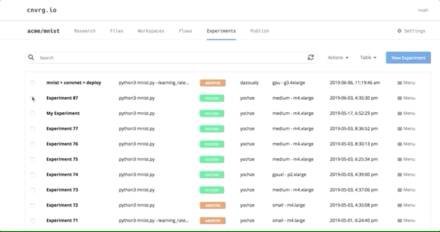
Running an experiment

On your project’s sidebar, click Experiments, then click New Experiment. In the panel that appears:

1. For Command to Execute, type in or select Rscript train.R.
2. For Environment > Compute, select medium.
3. For Environment > Image, click cnvrg_r and choose the latest cnrvg R image.
4. Click Submit.

TIP

There are plenty of other options that you can use when running an experiment that enable powerful experiments for any use case. see here

Now, cnvrg will get everything set up and start running the experiment. It might take a few minutes but on the experiment page you can follow its progress live. You can view the output and the graphs that are created.

You should also notice towards the top, all our cnvrg tags being populated and tracked.

Running a grid search

Our single training experiment is now complete. It looks pretty good, but maybe if we changed some of our parameters we could end up with a stronger model. Let’s try a grid search to find out.

cnvrg has native support for running any form of hyper-search, and it requires only making a couple changes to your code to support it.

The train.R file has been preprepared for grid searching, but let's have a look to see how it is accomplished.

Go back into the workspace that we set up (if you closed it, launch a new workspace the same way we did before).

All that is needed for grid searching, is to ensure we can parse the different parameters from the command line and use them as variables in the code.

The package we recommend using in R is optparse. You can see on line 14 that we have added that package for use:

library("optparse")

Lines 16 - 24 set up the correct usage of optparser:

# Set grid search options
option_list = list(
     make_option(c("--partition_size"), type="double", default=0.7,help="percent of dataset to become training set",metavar="number"),
     make_option(c("--folds"), type="integer", default=10,help="number of folds to perform",metavar="number")
     );

# Read parameters
opt_parser = OptionParser(option_list=option_list);
opt = parse_args(opt_parser);

You should also notice that at various relevant points, the variables are being used throughout the code.

Without any further ado, let's run a grid search!

Run a grid search

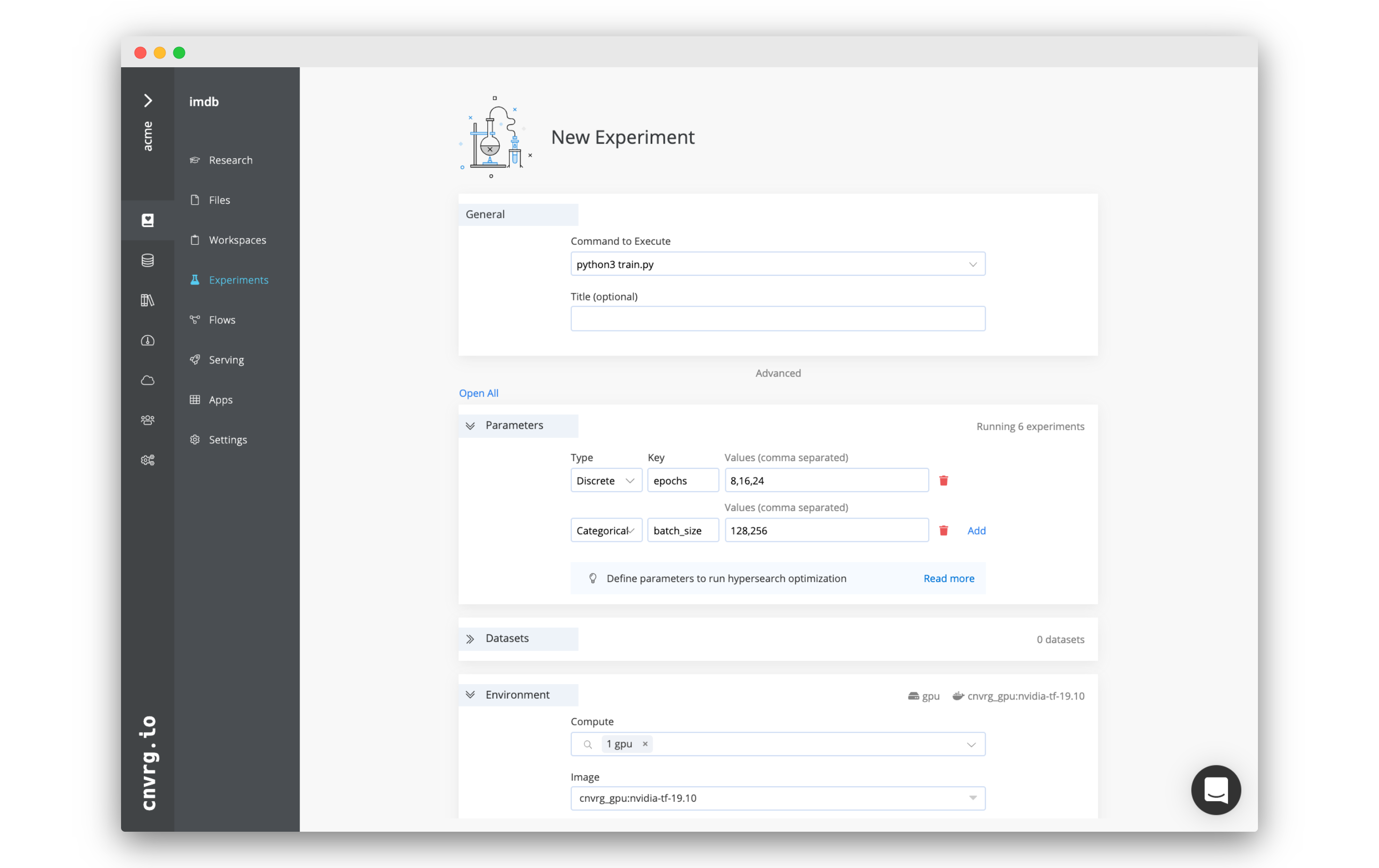
Go back to the Experiments tab. Click New Experiment. In the panel that appears:

1. For Command to Execute, type in or select Rscript train.R.
2. Click on the Parameters subsection. We will now add two parameters for the grid search.
   • Partition Size:
     • Type: Float
     • Key: partition_size
     • Min: 0.6
     • Max: 0.9
     • Scale: linear
     • Steps: 4
   • Folds (Click add to insert another parameter):
     • Type: Categorical
     • Key: folds
     • Values: 5,10,15
3. For Environment > Compute, select medium.
4. For Environment > Image, click cnvrg_r and choose the latest cnrvg R image.
5. Click Submit.

cnvrg will set up 12 discrete experiments and run them all using the hyperparameters as entered.

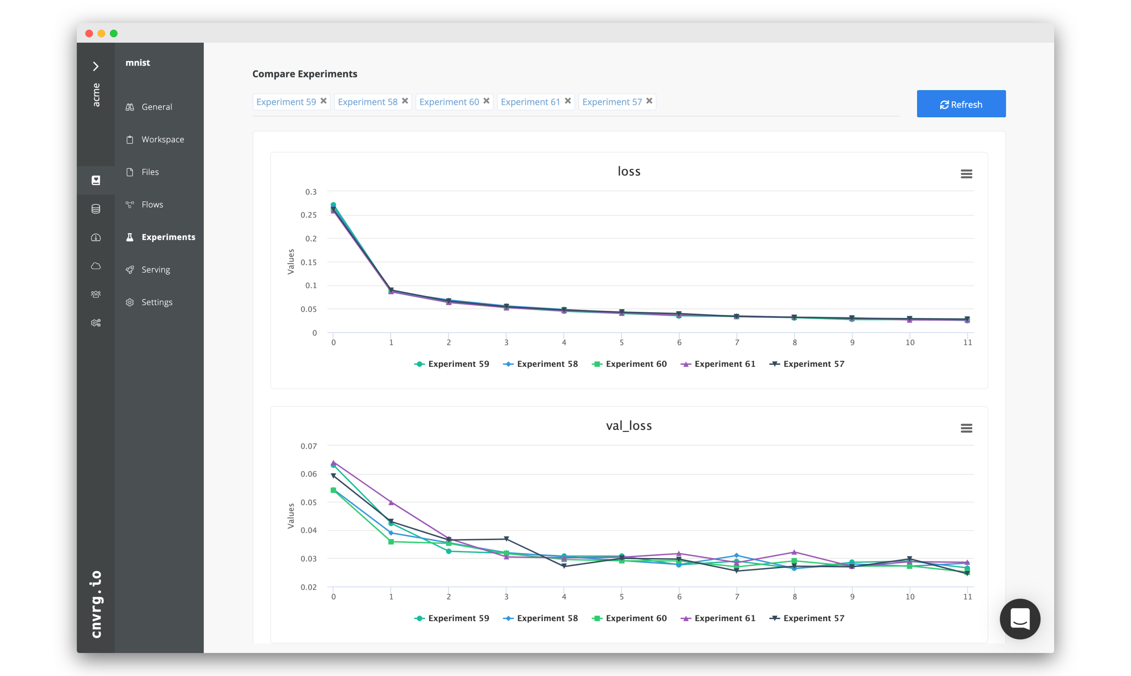
Visualizing and comparing

After all of our experiments have run successfully, we can now compare and choose the best performing model. Cnvrg makes this really easy with the built-in visualization and comparison tools.

Navigate back to the Experiments page and select all the experiments we just ran as part of the grid search. At the top, click Actions, then select Compare in the drop-down menu.

Here we can see all the results and metrics of our experiments beautifully displayed together. It makes it easier to choose our most accurate model.

This can be really useful for identifying the best experiment and model!

Conclusion

In this tutorial, we managed to run 13 different experiments, use R Studio and play around with cnvrg Research Assistant. You can use everything we did and extend it for your own code and projects.

Make sure to check out some of our other tutorials to learn more about cnvrg using different use cases. Maybe try using R Shiny next!